Prefer to play? This chapter is also an interactive Livebook where you drag the control points with sliders and watch the curve follow.
Points that pull
A Bezier curve is defined by a short list of points:
- The curve starts at the first point and ends at the last point.
- The points in between are control points. The curve doesn't go through them; it is pulled towards them, like a rope pulled by magnets.
Curves.define_bezier([{0, 0}, {1, 4}, {3, -1}, {4, 3}])The number of points decides the kind of curve:
| 2 points | 3 points | 4 points |
|---|---|---|
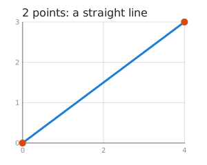 | 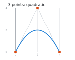 | 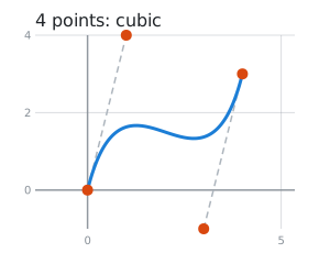 |
| A straight line: no control points. | Quadratic: one control point pulls on the whole curve. | Cubic: the first control point sets how the curve leaves the start, the second how it arrives at the end. |
The dashed lines join each control point to the end it pulls on. They show the direction the curve leaves the start, and the direction it arrives at the end.
How hard is the pull?
The further a control point is from the line, the harder it pulls. Here the start and end stay the same, and only the two control points move:
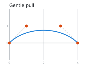 | 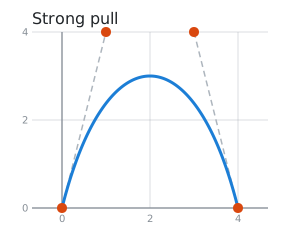 | 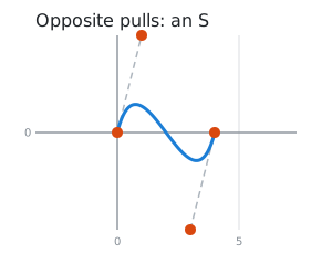 |
[{0, 0}, {1, 1}, {3, 1}, {4, 0}] | [{0, 0}, {1, 4}, {3, 4}, {4, 0}] | [{0, 0}, {1, 4}, {3, -4}, {4, 0}] |
When the two control points pull in opposite directions, you get an S.
You already know these: CSS easing
If you have written CSS, you have used cubic Bezier curves. transition-timing-function: cubic-bezier(x1, y1, x2, y2)
is a curve from {0, 0} to {1, 1} with the control points {x1, y1} and {x2, y2}. So you can copy any
CSS easing straight into Curves:
# cubic-bezier(0.68, -0.55, 0.27, 1.55), a bouncy "back" easing
curve = Curves.define_bezier([{0, 0}, {0.68, -0.55}, {0.27, 1.55}, {1, 1}])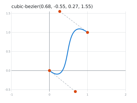
Control points can sit outside the 0..1 box. That makes the curve overshoot: it dips below 0 at the
start and goes past 1 before it settles.
Too many points?
A single Bezier curve takes 2 to 4 points. With more, solving it returns an error:
curve = Curves.define_bezier([{0, 0}, {1, 1}, {2, 0}, {3, 1}, {4, 0}])
Curves.solve(curve, 0.5)
#=> {:error, {:too_many_points, 5, 4}}
For longer paths, chain curves together with a spline.
Next: Splines.